1  Introduction

Learning Goals

• Familiarize yourself with the RStudio layout.
• Play around in the RStudio console to gain familiarity with the basic structure of R code.

1.1 Background

Data

The word data often brings spreadsheets to mind, like the following data on penguins.

# A tibble: 5 × 6
# Groups:   species, island [5]
  species   island    bill_length_mm bill_depth_mm flipper_length_mm body_mass_g
  <fct>     <fct>              <dbl>         <dbl>             <int>       <int>
1 Adelie    Biscoe              37.8          18.3               174        3400
2 Adelie    Dream               39.5          16.7               178        3250
3 Adelie    Torgersen           39.1          18.7               181        3750
4 Chinstrap Dream               46.5          17.9               192        3500
5 Gentoo    Biscoe              46.1          13.2               211        4500

This data is called tidy because:

• each row = a unit of observation (a penguin in this data).
• each column = a measure on some variable of interest: quantitative (numbers with units) or categorical (discrete possibilities or categories).
• each entry contains a single data value, ie, no analysis, summaries, footnotes, comments, etc. Only one value per cell.

Check Your Understanding

Considering the above data, answer the following questions:

• How many observation are there?
• How many measures are there? What are they?
• What is the bill length in mm of the Adelie penguin living in the Dream island?

The definition of data, however, is much more expansive, like this one from Google:

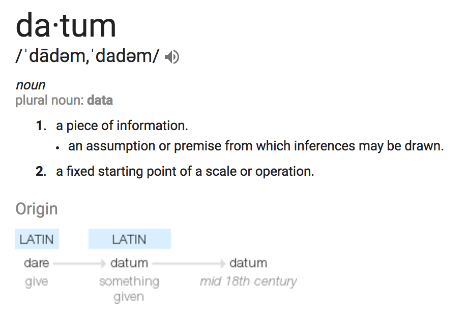
The followings are data, too!

1. emails in your inbox which contain text and more
2. social media posts which contain text and more
3. images
4. videos
5. audio files

Check Your Understanding

For each data example above, answer the following questions:

• How can the data be converted into a tidy table?
  • What are the units of observation, ie, what do the rows represent?
  • What are four of the possible variables we might track for each observation, ie, what goes into the columns?
• Indicate what people, groups, organizations, etc might use data like this.

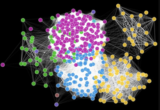
Data Science

Data Science extracts knowledge from data within a particular domain of inquiry, and particular contexts. Below are examples from just within Macalester:

• Robin Shields-Cutler (Biology) uses big data to study microbiomes.
• Xavier Haro-Carrión (Geography) uses satellite & remote sensing data to study biodiversity conservation.
• Lisa Mueller (Political Science) uses data to analyze political protest outcomes.
• John Kim + Futures North (Media & Cultural Studies) uses data-driven art to explore & illustrate migration patterns.
• Bethany Miller + Macalester’s Institutional Research team use data to better understand and shape everything from student outcomes to peer school comparisons.
• Macalester Athletics uses data to study everything from training outcomes to team performance to sleep patterns.

(a) Shields-Cutler’s website

(b) Haro-Carrión’s website

(c) the Futures North website

Figure 1.1: Images from faculty at Macalester

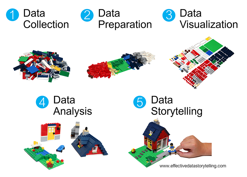
Data Science Workflow

Though the examples above vary dramatically in their domain, context, and methodology, they share a general data science workflow as shown below. We will touch on each of the steps of this workflow this semester.

Data Science workflow, as told through Legos. Source

Step	In 112	Beyond 112 (or as part of your project)
data collection	the basics of getting data into RStudio	web scraping, databases, APIs
data preparation	essential wrangling skills	advanced wrangling skills, natural language processing
data visualization	essential univariate, bivariate, multivariate, and spatial viz	interactive viz, animations
data analysis	exploratory data analysis	prediction, statistical modeling, machine learning, AI
data storytelling	yes!	yes!

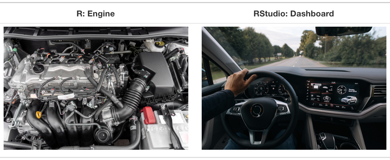
Software

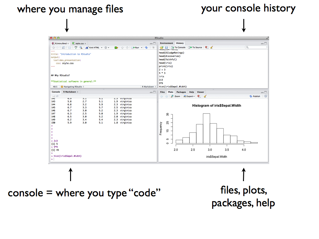
Working with modern data, hence doing Data Science, requires statistical software which means that calculators and spreadsheet functionality don’t cut it. Hence, We’ll exclusively use R and RStudio. Below are illustrative pictures of both.

Figure 1.1 from A ModernDive into R and the Tidyverse.

Why R?

• free
• open source–the code is free & anybody can contribute to it
• huge online community which is helpful for when we get stuck
• industry standard along with Python
• create reproducible and lovely documents including this online book!

Fun Fact

RStudio was started by 1991 Mac alum Joseph J. Allaire and beta-tested at Mac!

1.2 Exercises

Instructions

General

• Be kind to yourself.
• Collaborate with your assigned partner.
• Ask questions when you and your assigned partner get stuck.
• The best way to learn is to play around focusing on recognizing patterns then noting them down
• Remembering details could be challenging at the beginning but will become natural the more you code.
• The solution to the exercise is at the bottom of the page. Check your answers against it.

Launching RStudio

Your portfolio should be opened in RStudio as a project. Check the upper-right corner of RStudio, if your portfolio repository name is shown there, then your are good to go. Otherwise, open GitHub Desktop –> from dropdown menu located on the top-left corner, select your portfolio repository if not selected –> Repository menu –> select Show in Explorer/Finder → double-click the file ending in Rproj

Adding Lesson to Portfolio

NOTE: If the lesson does NOT requires creating a Quarto document, skip the following instructions.

1. Your portfolio Quarto book project contains qmd files inside the ica folder for some of the lessons. If there is one for this lesson, open it. Otherwise, create a new Quarto document inside the ica folder then include it in the _quarto.yml file in the appropriate location. Ask the instructor if you could not figure out this step.
2. Click the </> Code button located at the top of this page and copy only the code where the Exercises section starts into the Quarto document of the lesson and solve the exercises. You can also Use your Quarto document to take notes. NOTE: If the code you copied contain reference to other Quarto documents, ie, {{< another_quarto.qmd >}}, remove them. otherwise, you code will not render.

Exercise 1: RStudio

Launch RStudio. Notice that there are four panes, each serving a different purpose. Today, we’ll work within the console and will not save any work.

Figure 1.2: RStudio Interface

Problem with RStudio?

If you have problem running RStudio on your machine, you can temporarily use Mac’s RStudio server after logging in using your Mac credentials.

Exercise 2: Console

We can use RStudio to do simple calculations using R. Type the following lines in the console, one by one, hitting Return/Enter after each. Take note of what you get. In some cases you might get an error! This error is important to learning how R code does and doesn’t work.

4 + 2
4/2
4^2
4*2
4(2)

Check

Check with your partner.

Exercise 3: Functions

Having a calculator is nice, but we’ll typically use built-in functions to perform common (repetitive) and specific tasks. These functions have names and require information, called arguments, in order to run. Functions are called as follows:

function(argument)

Try out the following functions in the console. Note each function’s name, argument (information it needs to run), and output (i.e. what the function does and produce):

sqrt(9)
sqrt(25)
nchar("snow")
nchar("macalester")
sqrt(nchar("snow"))

Some functions require more than 1 argument, separated by commas. To keep these straight, we often specify the arguments by name as follows:

function(argument1 = ___, argument2 = ___)

Try out the following functions in the console. Note each function’s name, argument (information it needs to run), and output (i.e. what the function does and produce):

rep(x = 2, times = 5)
rep(times = 5, x = 2)
rep(2, 5)
rep(5, 2)
seq(from = 2, to = 10, by = 2)
seq(2, 10, 2)
seq(from = 2, to = 10, length = 3)
seq(2, 10, 3)

Note that R is case-sensitive. Try the following code which uses Seq() instead of seq() (capital case S instead of lower case s). Read the error message and make sure to understand it–you will experience this type of error message a lot! It will happen any time you misspell a function among other reasons we’ll experience later.

Seq(2, 10, 3)

Exercise 4: Grammer

We’ll learn lots and lots of functions this semester. Nobody has every function memorized. That said, it does help to connect function names with their purpose. Do that for each function you used above.

• sqrt() = square root
• nchar() = ???
• rep() = ???
• seq() = ???

Check

Check with your partner.

Exercise 5: Practice

Use the functions you learned above to do the following:

• Count the number of letters in the word data.
• Create the sequence 3, 6, 9, 12–do it in more than one way.
• Create a sequence of 4 numbers that start at 1 and end at 10–do it in more than one way.
• Repeat the number 5 8 times.
• Produce the sequence 3, 6, 9, 12, 3, 6, 9, 12–you need to combine 2 functions

Exercise 6: Variables

For reasons that will become clear in the future, we’ll often want to store some R output for later. We can so so using the assignment operator as follows:

name <- output

In the above assignment statement:

• name is the name under which to store a result
• output is the result we wish to store
• <- is the assignment operator–you can think of this as an arrow pointing the output into the name.

Try out each line one at a time. Some lines will not show any output. Why?

degrees_c <- -13
degrees_c

Let’s now use what we stored. Again, do this one by one.

degrees_c * (9/5) + 32
degrees_f <- degrees_c * (9/5) + 32
degrees_f

Finally, try to print degrees_tomorrow. Take time to read the error message. You will experience this type of error message a lot! It will happen when you either haven’t yet defined the object you’re trying to use or you’ve misspelled its name among other reasons we’ll experience later.

degrees_tomorrow

Check

Check with your partner.

Exercise 7: Practice

• Name and store your current age in years.
• Confirm that your age is stored correctly by typing the name and pressing return/enter.
• Use your stored age to calculate how old you’ll be in 17 years.

Exercise 8: Code Styling

It’s important to recognize that code is a form of communication, both to yourself and others. Code structure and details are important to readability and clarity just as grammar, punctuation, spelling, paragraphs, and line spacing are important in written essays. All of the code below works, but has bad structure. Discuss with your partner what is unfortunate about each line.

seq(from=1,to=9,by=2)
seq(from = 1, to=9,by=2)
my_output <- -13
thisisthetemperaturetodayincelsius <- -13
this_is_the_temperature_today_in_celsius <- -13

When writing code, avoid smooshy ones similar to the following:

# BAD: tough to read
seq(from=1,to=9,by=2)

# GOOD: spaces between "words" and punctuation helps
seq(from = 1, to = 9, by = 2)

When naming your variables:

• use meaningful names,
• make them short if possible
• split up multiple-word names using snake_case or camelCase

# BAD: too smooshy and hard to read
degreescelsius <- -13

# BETTER but not the R-way of naming variables
# Why is it called camel case?
degreesCelsius <- -13

# BETTER
degrees_celsius <- -13

It’s also impossible, not just ill-advised to start names with numbers or symbols, or to use certain symbols in our names. Try the followings:

1_18_24_degrees_c <- -13
_degrees_c <- -13
Jan/18/24/degrees <- -13

Exercise 9: Mistakes & Help

Mistakes are common when learning any new language. You’ll get better and better at interpreting error messages, finding help, and fixing errors. These are all important skills in computer programming in general.

Console Shortcut

With your cursor at the next prompt in the console (>), press the up arrow multiple times. What does this do?! This shortcut will be very handy when you make mistakes and want to modify your code without having to start over.

Help Files

You’ll often forget how functions are used. Luckily, there’s typically built-in documentation for built-in functions that can be invoked using the ? operator.

Let’s practice:

• In the console, type ?rep and press return/enter.
• Check out the documentation file that pops up in the Help pane.
• Quickly scroll through, noting the type of information provided.
• Stop at the Examples at the bottom. Perhaps the most useful section, this is where a function’s functionality is demonstrated! Try out a couple of the provided examples in your console.

Exercise 10: History & Environment

Finally, let’s leave the console.

• Check out the Environment pane of RStudio. What do you observe there and when might this be helpful?
• Similarly, check out the History pane of RStudio. What do you observe there and when might this be helpful?

Optional Excersise: Watch Explaination

If you’ve finished the above exercises, you can watch Dr. Alicia Johnson talks through the concepts learned today (YouTube).

1.3 Solutions

Click for Solutions

Exercise 2: Concole

4 + 2

[1] 6

4/2

[1] 2

4^2

[1] 16

4*2

[1] 8

# This code gives an error! Multiplication requires *
4(2)

Exercise 3: Functions

# sqrt calculates square root
sqrt(9)

[1] 3

sqrt(25)

[1] 5

# nchar counts up the number of characters
nchar("cat")

[1] 3

nchar("macalester")

[1] 10

# rep repeats the value "x" the number of "times" indicated
# Order doesn't matter
rep(x = 2, times = 5)

[1] 2 2 2 2 2

rep(times = 5, x = 2)

[1] 2 2 2 2 2

# We don't need to label the arguments
# But the order matters! It assumes an order of "x" then "times"
rep(2, 5)

[1] 2 2 2 2 2

rep(5, 2)

[1] 5 5

# Create a sequence of numbers
# Removing the argument labels gives the same result 
seq(from = 2, to = 10, by = 2)

[1]  2  4  6  8 10

seq(2, 10, 2)

[1]  2  4  6  8 10

# We can also define a sequence by its length, not increments
# But can't remove the argument labels (R assumes the 3rd argument is length)
seq(from = 2, to = 10, length = 3)

[1]  2  6 10

seq(2, 10, 3)

[1] 2 5 8

Exercise 4: Grammer

• sqrt() = square root
• nchar() = number of characters
• rep() = repeat / repetition
• seq() = sequence

Exercise 5: Practice

# Count the number of letters in "data"
nchar("data")

[1] 4

# Create the sequence 3, 6, 9, 12
seq(from = 3, to = 12, by = 3)

[1]  3  6  9 12

seq(from = 3, to = 12, length = 4)

[1]  3  6  9 12

# Create a sequence of 4 numbers that start at 1 and end at 10
seq(from = 1, to = 10, length = 4)

[1]  1  4  7 10

seq(from = 1, to = 10, by = 3)

[1]  1  4  7 10

# Repeat the number "5" 8 times
rep(x = 5, times = 8)

[1] 5 5 5 5 5 5 5 5

rep(5, 8)

[1] 5 5 5 5 5 5 5 5

# Combine 2 functions to produce the sequence 3, 6, 9, 12, 3, 6, 9, 12
rep(x = seq(from = 3, to = 12, by = 3), times = 2)

[1]  3  6  9 12  3  6  9 12

Exercise 6: Variables

degrees_c <- -13
degrees_c

[1] -13

degrees_c * (9/5) + 32

[1] 8.6

degrees_f <- degrees_c * (9/5) + 32
degrees_f

[1] 8.6

Exercise 7: Practice

my_age <- 20
my_age

[1] 20

my_age + 17

[1] 37

Exercise 8: Code Styling

# This is too smooshy and hard to read
seq(from=1,to=9,by=2)

# The use of spacing is inconsistent, hence hard to read
seq(from = 1, to=9,by=2)

# Too vague
my_output <- -13

# Too smooshy
thisisthetemperaturetodayincelsius <- -13

# Easier to read, but too long
this_is_the_temperature_today_in_celsius <- -13

Exercise 10: History & Environment

• Environment: shows what objects you’ve stored (eg: degrees_c)
• History: shows what R code you’ve typed